Browse

2023 2022

The Journal of Digital Assets

Volume 1
December 2022
Issue 1

Articles

Impermanent Loss and Gain of Four Automated Market Maker Algorithms
Hyoung Joong Kim, Soohyuk Choi, Yong Tae Yoon, and Shiyong Yoo
First Published: 05 December 2022
Abstract | Full Text(662) | PDF download(217)

Content (Full Text)

Impermanent Loss and Gain of Four Automated Market Maker Algorithms

Hyoung Joong Kim, Soohyuk Choi, Yong Tae Yoon, and Shiyong Yoo

Abstract

Automated market makers are working without an order book, and they determine the price of assets automatically. It is reported that he automated market makers have the impermanent loss, which causes financial damage to liquidity providers. Impermanent loss makes the liquidity providers hesitant to deposit assets in the liquidity pool. Therefore, their participation incentive from liquidity provision should be anticipated by automatic market makers inherently. However, the existence of impermanent gain has never been reported. Impermanent gain is important to attract liquidity providers without giving compensation incentives. This study shows that for some automated market makers, impermanent gain coexists with impermanent loss. Examples showing the coexistence and conditions are provided.

Keywords: Blockchain, cryptocurrency, decentralized finance, impermanent gain, impermanent loss, market maker.

I. INTRODUCTION

BLOCKCHAIN[1][22]is an important building block for many applications, including smart grid [2][13], energy trading[15], vehicular device[1], cryptocurrency[23], voting[14], education system[20], identity authentication[5], and decentralized finance (DeFi). Among the applications, DeFi has grown explosively from 2020, securing credibility and liquidity. These DeFi services include lending, asset management, and decentralized exchange. An automated market maker (AMM) is a crucial part of the DeFi ecosystem, in particular, for the decentralized exchange systems. Meanwhile, AMMs rely on mathematical formulas to facilitate trading and automatically set the price of an asset or multiple assets. AMMs of the decentralized exchanges recently have replaced the traditional order book so that all trades are conducted through swaps on their liquidity pools. AMMs allow the users to buy and sell in real-time without matching orders. The buyand-sell orders listed in the order book are arranged by price. Moreover, the price of the assets at an exchange is set by the matching order algorithms, such as price-time priority algorithm or price pro-rata

This research was supported by a grant of the Korea Health Technology R&D Project through the Korea Health Industry Development Institute (KHIDI), funded by the Ministry of Health & Welfare, Republic of Korea (grant number: HI19C0785).

This paper is an extension of the prepublication available at [10].

H. J. Kim is with the School of Cybersecurity, and the Cryptocurrency Research Center, Korea University, Seoul, 02841, South Korea (e-mail: khj-@korea.ac.kr).

S. Choi is with the SymVerse, Seoul, 02841, South Korea (e-mail: choi@symverse.com).

Y. T. Yoon is with the Department of Electrical and Computer Engineering, Seoul National University, Seoul, 08826, South Korea (e-mail: ytyoon@snu.ac.kr).

S. Yoo is with the Business School, Chung-Ang University, Seoul, 06974, South Korea (e-mail: sy61@cau.ac.kr).

Corresponding author: H. J. Kim

Received: August 25, 2022; Revised: October 15, 2022; Published: December 5, 2022.

ISSN : 2951-5181

DOI : 10.23164/journal.221205.000001

algorithm. It is determined by double auction. Sellers and buyers can offer market, limit, or conditional orders on the centralized exchanges. Meanwhile, the AMMs have provided the decentralized exchanges mathematical price valuation models. As those formulas are adopted, market makers are price setters, whereas traders are price takers. That is to say, sellers and buyers have no choice but to accept the price determined by the market maker.

Wang[21]suggested the following requirements to be a good AMM algorithm. Constant function market maker (CFMM) needs to be convex curves or convex hyperplanes to conform to the principle of supply and demand. Another requirement is the robustness against malicious attacks, such as front-running (slippage) attacks [7][8]. Front-running is an action plan where an attacker benefits from prior access to privileged market information about upcoming transactions and trades[7]. Wang[21]also suggested the computational efficiency of the asset amount determination.

Meanwhile, Hanson [9][10] has proposed market-scoring rule for the market prediction. Recently, Hanson’s market-scoring rule, the ogarithmic market scoring rule (LMSR), showed the potential of the AMM tool. LMSR is one of the CFMM and AMMs. Note that the LMSR is quite popular because of the following three reasons [17]: (1) it was the first AMM for prediction markets and decentralized exchanges; (2) it has a simple analytical form that is rather complicated than constant function market makers; and (3) it has bounded loss.

Othman et al. [18] have proposed liquidity-sensitive LMSR (LS-LMSR) by introducing a parameter and adaptive to the market situation; they aim to make the scoring liquidity sensitive. The LMSR and LS-LMSR algorithms set the price of a cryptocurrency pair by keeping the constant cost value unchanged. A logarithmic function expresses the cost. A bonding curve is a mathematical curve that defines a relationship between price and supply of assets. Bonding curve (between two assets as a pair, such as ETH and USDC, where the ETH is a cryptocurrency with price volatility, and the USDC is a stablecoin) or bonding hyperplane (for more than two assets) can be used for setting the price.

CFMM [2] sets the price by maintaining the cost value unchanged (i.e., equal to a constant). Other types of algorithms, such as constant product market maker (CPMM) algorithm [4], constant sum market maker (CSMM) algorithm, and constant mean market maker (CMMM) algorithm [12], also set the price in such a way that the cost value remains unchanged over the bonding curves or bonding hyperplanes. Meanwhile, a hybrid approach called StableSwap [6] combines the CPMM and CSMM algorithms to take the advantages of both methods. Constant circle market maker (CCMM) and constant ellipse market maker (CEMM) also do similar thing.

Liquidity providers supply asset pairs to the liquidity pool, and they may lose money and suffer from an impermanent loss (a.k.a. divergent loss). Impermanent loss is the temporary loss of asset values occasionally experienced by liquidity providers because of volatility in a trading pair. Liquidity provider’s asset value can be increased or decreased after trading. The composition ratio of assets is changed, and, as a result, the asset price and value are changed after asset trading. Impermanent loss occurs when the deposited asset value is decreased; it is still a loss, whether large or small. This loss is impermanent because it can only be temporary.
If the impermanent loss is large, liquidity providers are strongly hesitant to supply liquidity to the liquidity pool. Moreover, the loss disappears when the composition ratio of the assets returns to the original ratio deposited by the liquidity provider. Impermanent loss is a hot topic and has been studied [3][4][6][7][11][12] [16][18][21].

The contributions of this paper can be summarized as follows. To the best of our knowledge, this study is the first to show that impermanent gain and impermanent loss coexist for some AMMs. Previous study has already shown that CPMM has the property of impermanent loss [12]. Meanwhile, this present study shows that the CPMM does not have impermanent gain property at all. Moreover, it was known that CSMM does not have the property of impermanent loss because the price is invariant. However, this study shows that the relative price in the CSMM is not invariant, and the CSMM has both the property of impermanent gain and impermanent loss. For the LS-LMSR and CCMM and AMMs, this study also shows that both impermanent gain and impermanent loss coexist.

This paper is organized as follows. Section 2 introduces real-world examples and the mathematical background of various AMM asset cost functions and asset value functions to define the value difference functions, which indicates impermanent loss and impermanent gain. Section 3 derives the condition to obtain an impermanent gain and shows that impermanent gain can coexist with impermanent loss. Section 4 concludes the paper with some suggestions.

II. MATHEMATICAL BACKGROUND WITH AN EXAMPLE

Consider an example that explains the impermanent loss or impermanent gain in an easy to understand way. There are 10 ETH and 1,000 USDT in pairs deposited in a liquidity pool (LP). In this particular AMM, the deposited token pair needs to be of equivalent value. This means that the price of ETH is 100 USDT at the time of deposit. This also means that the dollar value of the total deposit is 2,000 USD at the time of deposit since she has 10 ETH for 1,000 USD and 1,000 USDT for 1,000 USD as well. In this paper, it is assumed that one of the coin pairs deposited in the LP is a stablecoin and the other is a non-stablecoin. In the LP, there is a pair of coins $x$ and $y$ where $x$ and $y$ denote the number of ETH and USDT, respectively. Hence, the price of $x$ is determined by $P = y / x$ , and the total value of the assets in the pool is given as $V = ((\frac{y}{x}) x + y) = 2 y$ .

(Case 1) In this LP, the coin price is determined by the AMM algorithm satisfying the simple equation $x y = k$ where $k$ is a fixed constant. At the initial moment, since there were 10 ETH and 1,000 USDT, $k$ is obviously 10,000 such as (10 ∙ 1,000 = 10,000). Now, Alice sold 1 ETH at the pool. Since $x$ has to be changed from 10 to 11, $y$ has to be decreased from 1,000 to approximately 909.09 to keep $k$ unchaged. After the swapping, the price of ETH has been changed from 100 USD to approximately 82.64 USD. Thus, total asset value of the LP has been changed from 2,000 USD to 1,818.18 USD.

Assuming that the liquidity provider who deposited 10 ETH and 1,000 USDT did not participate in the LP, he calculated the value of his assets at the current coin price. Since the current ETH price has fallen to 82.64 USD, his asset value is 1,826.4 USD by adding 826.4 USD from his original 10 ETH and 1,000 USD from his original 1,000 USDT. He realized that by becoming a liquidity provider, his current asset value is 1,818.18 USD, but if he had not participated in the LP, it would have been close to 1,826.4 USD, resulting in a loss of 8.22 USD. The AMM algorithm of the LP is CPMM one. This loss is called impermanent loss because it does not always occur. Impermanent loss is also called divergence loss.

(Case 2) Let’s consider another example. In another LP, the coin price is determined by the AMM algorithm satisfying the simple equation $x + y = k$ where $k$ is a fixed constant. At the initial moment, since there are 10 ETH and 1,000 USDT, $k$ is obviously 1,010 such as (10 + 1,000 = 1,010). Now, Bob sold 1 ETH at the pool. Since $k$ hasto be changed from 10 to 11, $y$ hasto be decreased from 1,000 to 999 to keep $k$ unchaged. After the swapping, the price of ETH is changed from 100 USD to approximately 90.8 USD. Thus, the total asset value of the LP is still 2,000 USD. If he had not participated in the LP, his asset value would be 908 USD from 10 ETH and 1,000 USD from the original 1,000 USDT, adding up to 1,908 USD. Thus, he made a gain of 92 USD by participating in the LP running CSMM AMM. This gain is called impermanent gain or divergence gain. CSMM AMM has always been known to have zero divergence loss, but from this example it seems clear that this is not the case and positive divergence gain certainly exists.

The difference between the claim that the divergence loss of CSMM is always 0 and that it can be positive sometimes comes from the difference in the definition of the divergence loss. In the above example, the initial asset value of CSMM LP and that after swapping are the same at 2,000 USD. Therefore, the difference in the asset value of CSMM LP before and after a certain swapping is always zero. If the definition of divergence loss is defined as the value obtained by subtracting the initial asset value from the asset value after swapping, it is true that the divergence loss of CSMM LP is always 0. However, in this paper, divergence loss is defined as the difference between the asset value after swapping and the value of the initial asset converted to the price after swapping. The difference of the definitions is clear; see Equation (4) in [12] and also Equation (4) in this paper. In calculating the total asset value, the former considers both the asset pairs and prices before and after the swapping, whereas the latter considers the initial asset pair and the price before and after the swapping.

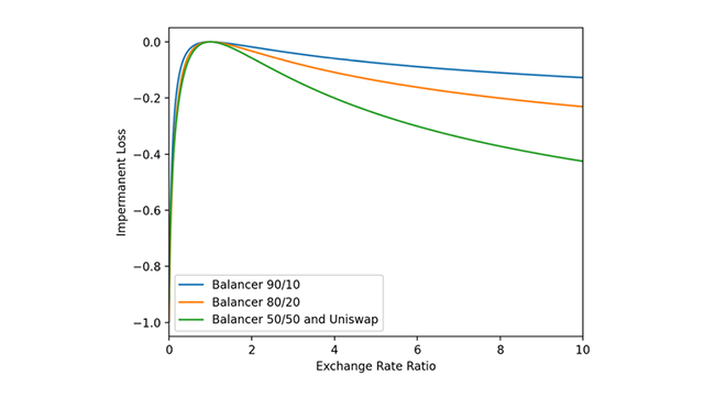
(Case 3) See the same example of CPMM LP given above. At the initial moment, since there were 10 ETH and 1,000 USDT, $k$ is 10,000. Now, Carol bought 1 ETH from the pool. Since $x$ has to be chan gefrom 10 d to 9, $y$ has to be increased from 1,000 to approximately 1,111.11 to keep $k$ unchaged. After the swapping, the price of ETH has been changed from 100 USD to approximately 123.46 USD. Thus, total asset value of the LP has been changed from 2,000 USD to 2,222 USD. According to Equation (4) in [12], the divergence loss is 222 USD (i.e., 2,222−2,000) which is positive. Impermanent loss is known to be non-positive as shown 1 Figure 1 [19], but here it is positive, so it goes against common sense.

On the other hand, according to Equation (4) in this paper, the divergence loss is −13 USD (i.e., 2,222−2,235) which is negative. This case conflicts with reports that the CPMM divergence loss is nonpositive (see Figure 1). Table 1 illustrates the mechanism by which impermanent loss occurs.

Fig. 1. Impermanent loss for Uniswap and Balancer pools compared [19].

Table 1. The mechanism by which impermanent loss occurs.

Consider a pair of two assets where $q_{t} (x_{t}, y_{t})$ denotes the asset pair with the number of assets $x$ and $y$ at time $t$ . The AMM uses a cost function $C (q_{t})$ to set the price of cryptocurrency pairs at a trading. Suppose a liquidity provider has deposited an asset pair $(x_{0}, y_{0})$ , where the asset $y$ is a stablecoin. Note that $y$ is considered a unit of account because it is a stablecoin; it is also divisible, fungible, and countable. Its price is unity.

Then, the asset value of the liquidity provider at time 0 is given as follows:

V (q_{0} (x_{0}, y_{0})) = \frac{y_{0}}{x_{0}} \cdot x_{0} + y_{0} = 2 y_{0}

(1)

Composition ratio of the two assets is changed from

(x_{0}, y_{0})

(x_{n}, y_{n})

by trading two assets. One can add

δ x

to the pool to make

x_{n} = x_{n - 1} + δ x

; thus,

y_{n} = y_{n - 1} - δ y

. Similarly, one can add

δ y

to the liquidity pool to make

y_{n} = y_{n - 1} + δ y

; hence,

x_{n} = x_{n - 1} - δ x

. The asset value of the pair

(x_{n}, y_{n})

at time

t

is computed as follows:

V (q_{n} (x_{n}, y_{n})) = \frac{y_{n}}{x_{n}} \cdot x_{n} + y_{n} = 2 y_{n}

(2)

However, the value of the original pair composition

(x_{0}, y_{0})

assessed by the relative price

\frac{y_{n}}{x_{n}}

at time

n

is computed as

V (q_{n} (x_{0}, y_{0})) = \frac{y_{n}}{x_{n}} \cdot x_{0} + y_{0}

(3)

In addition, impermanent loss is computed from the difference

D

of the two asset values

V (q_{n} (x_{n}, y_{n}))

and

V (q_{n} (x_{0}, y_{0}))

, such that

D (x_{n}) = V (q_{n} (x_{n}, y_{n})) - V (q_{n} (x_{0}, y_{0}))

(4)

If the value of $D$ is negative, there exists an impermanent loss. Many research works [3][4][6][7][11][12][16][18][21] have tackled the impermanent loss. Scholars have tried eliminating or mitigating the impermanent loss. If the value of $D (x_{n})$ is positive, an impermanent gain exists. This paper introduces the concept of impermanent gain for the first time.
The exact definition of impermanent loss should be $D (x_{n}) = V (q_{n} (x_{n}, y_{n})) - V (q_{n} (x_{0}, y_{0})) = 2 y_{n} - ((y_{0} / x_{0}) \cdot x_{n} - y_{n})$ as in Equation (4). Note that some papers have defined the impermanent loss as $D (x_{n}) = V (q_{n} (x_{n}, y_{n})) - V (q_{n} (x_{0}, y_{0})) = 2 y_{n} - 2 y_{0}$ which is not correct.

A. Constant Product Market Maker

CPMM starts from the cost function from the product of

x_{0}

and

y_{0}

, such as

C (q_{0} (x_{0}, y_{0})) = x_{0} \cdot y_{0} = k

(5)

At time

n

, the number of

y_{n}

given

x_{n}

is computed from the following equation

C (q_{n} (x_{n}, y_{n})) = x_{n} \cdot y_{n} = k

(6)

Note that the CPMM cost function is a hyperbola. Uniswap, a decentralized exchange, uses this formula for a pricing purpose.
One can add

δ x

to the pool to make

x_{n} = x_{n - 1} + δ x

; then,

y_{n} = y_{n - 1} - δ y

. The cost function in Equation (6) is used to determine

δ y

by using

y_{n} = k / x_{n} = k / (x_{n - 1} + δ x)

and obtaining

δ y

by subtraction such that

δ y = y_{n} - y_{n - 1}

.
Hence,

y_{n}

is computed from Equation (6) as follows:

_{y_{n} = \frac{k}{x_{n}}}

(7)

For the CPMM, the relative price of asset

x

with respect to

y

at time

n

is computed from Equations (2) and (7):

p_{n} = \frac{y_{n}}{x_{n}} = \frac{k}{{x_{n}}^{2}}

(8)

Thus, the asset value of the pair

(x_{n}, y_{n})

at time

t

is computed from Equations (2) and (7) as follows:

V (q_{n} (x_{n}, y_{n})) = 2 \cdot \frac{k}{x_{n}}

(9)

Hence,

D (x_{n})

of the CPMM is computed from Equations (2),(3),and(9):

D (x_{n}) = 2 \cdot \frac{k}{x_{n}} - (\frac{k}{{x_{n}}^{2}} \cdot x_{0} + y_{0})

(10)

B. Liquidity-Sensitive Logarithmic Market Scoring Rule

Similarly, for the LMSR and LS-LMSR, the cost function is given as follows:

C (q (x_{n}, y_{n})) = b \cdot \ln (e^{x_{n / b}} + e^{y_{n / b}}) = k

(11)

Hence,

y_{n}

is computed from Equation (11):

y_{n} = b \cdot \ln (e^{k / b} + e^{x_{n / b}})

(12)

Thus, the asset value of the pair

(x_{n}, y_{n})

at time

t

is computed from Equations (2) and (12) as follows:

V (q_{n} (x_{n}, y_{n})) = 2 \cdot b \cdot \ln (e^{k / b} + e^{x_{n / b}})

(13)

For the LS-LMSR, the relative price of the asset

x

with respect to

y

is at time

n

is computed as:

p_{n} = \frac{y_{n}}{x_{n}} = b \cdot \ln (e^{\frac{k}{b}} - e^{\frac{x_{n}}{b}}) / x_{n}

(14)

C. Constant Sum Market Maker

For the CSMM, the cost function is given as follows:

C (q (x_{n}, y_{n})) = x_{n} + y_{n} = k

(15)

Hence,

y_{n}

is computed from Equation (15) as follows:

y_{n} = k - x_{n}

(16)

Thus, the asset value of the pair

(x_{n}, y_{n})

at time

t

is computed from Equations (2) and (16) as follows:

V (q_{n} (x_{n}, y_{n})) = 2 \cdot (k - x_{n})

(17)

D. Constant Circle Market Maker

CCMM has been proposed by Wang [21]. For the CCMM, the relative price and the change in the asset values are computed with the given cost function as follows:

C (q_{n} (x_{n}, y_{n})) = {(x_{n} - a)}^{2} + {(y_{n} - b)}^{2} = k

(18)

Hence,

y_{n}

is computed from Equation (18) as follows:

y_{n} = \sqrt{k - {(x_{n} - a)}^{2}} + b

(19)

Thus, the asset value of the pair

(x_{n}, y_{n})

at time

t

is computed from Equations (2) and (19):

V (q_{n} (x_{n}, y_{n})) = 2 \cdot (\sqrt{k - {(x_{n} - a)}^{2}} + b)

(20)

III. IMPERMANENT LOSS AND IMPERMANENT GAIN

The asset value difference is a good barometer to show whether there is impermanent loss. The difference value

D (x_{n})

is calculated from Equations (2) and (3) as follows:

D (x_{n}) = 2 y_{n} - (\frac{y_{n}}{x_{n}} x_{0} + y_{0})

(21)

Equation (21) is simplified:

D (x_{n}) = (2 - \frac{x_{0}}{x_{n}}) y_{n} - y_{0}

(22)

If $D (x_{n})$ is zero, then impermanent loss does not exist. A negative $D (x_{n})$ denotes impermanent loss, whereas a positive $D (x_{n})$ denotes impermanent gain. The sign of the difference $D (x_{n})$ is determined by Equation (22)

Theorem 1: If $x_{n} = x_{0}$ , then $D (x_{n})$ is zero, no matter what AMM is used

Proof: If $x_{n} = x_{0}$ , then $y_{n} = y_{0}$ . Thus, from Equation (22), when $x_{n} = x_{0}$ and $y_{n} = y_{0}$ , then $D (x_{n})$ is zero regardless of the type of AMM.

A. Constant Product Market Maker

For the CPMM, the CPMM AMM has the property of impermanent loss because showing that the sign of

D (x_{n})

is nonnegative is easy. For the CPMM,

D (x_{n})

is computed from Equations (7) and (22) as follows:

D (x_{n}) = (2 - \frac{x_{0}}{x_{n}}) (\frac{k}{x_{n}}) - (\frac{k}{x_{0}})

(23)

Note that

D (x_{n})

in Equation (23) is rewritten as

D = \frac{1}{{x_{n}}^{2}} [- (\frac{k}{x_{0}}) {x_{n}}^{2} + 2 k x_{n} - k x_{0}]

(24)

Equation (24) contains a quadratic function of

x_{n}

inside the square brackets. Note that the determinant ∆ of the quadratic function is zero. It implies that

D (x_{n})

is convex upward; hence, its maximum value is zero. Thus, we can easily show that

D (x_{n})

is always negative except for

x_{n} = x_{0}

no matter what the values of

x_{n}

x_{0}

, and

k

are. For

x_{n} = x_{0}

D (x_{n})

is zero. It implies that CPMM AMM never has the property of impermanent gain. The CPMM liquidity providers always have high chance of losing money. Thus, liquidity providers do not want to provide their assets to the liquidity pool if they are not given enough incentives to offset the losses.

B. Constant Sum Market Maker

The number of assets for the CSMM AMMs is determined by Equation (15). The price of

x_{n}

is determined as

p_{n} = \frac{y_{n}}{x_{n}} = \frac{k - x_{n}}{x_{n}}

(25)

Here, note that the relative price of

x_{n}

is varying because the relative price is a function of

x_{n}

, as shown in Equation (25). The range of the relative price

p_{n}

is (0, ∞) because the domain of

x_{n}

is (0,

k

). Thus, the price of

x_{n}

is varying, and not a constant, which contradicts existing research works [12].

For the CSMM, from Equations (15) and (22),

D (x_{n})

is computed as follows:

D = (2 - \frac{x_{0}}{x_{n}}) (k - x_{n}) - (k - x_{0})

(26)

Note that

D (x_{n})

in Equation (26) is rewritten as

D = \frac{1}{x_{n}} [- 2 {x_{n}}^{2} + (k + 2 x_{0}) x_{n} - k x_{0}]

(27)

Fig. 2. Loss and gain regions of three AMMs

Equation (27) contains a quadratic function of

x_{n}

inside the square brackets. Note that the determinant ∆ of the quadratic function is given as ∆=

{(k - 2 x_{0})}^{2}

. The determinant shows us two important facts. The first fact is that both impermanent loss and impermanent gain coexist for

x_{0}

≠

k / 2

. The second fact is that only impermanent loss exists for

x_{0}

k / 2

. Thus, we can easily show that

D (x_{n})

can be either positive or negative or zero, depending on the values of

x_{n}

x_{0}

, and

k

. When Equation (27) has two roots

x_{n}

k / 2

and

x_{n} = x_{0}

,both impermanent loss and impermanent gain coexist.

Theorem 2: If

x_{0}

≠

k / 2

, then CSMM AMM has the property of impermanent gain for

x_{0} < x_{n} < k / 2

k / 2 < x_{n} < x_{0}

Proof: See the paragraph above the Theorem 2.

Observation 1: If

x_{0} = y_{0} = k / 2

, CSMM AMM for Equation (15) has an impermanent loss property only for all

x_{n}

and

y_{n}

, which are both positive.

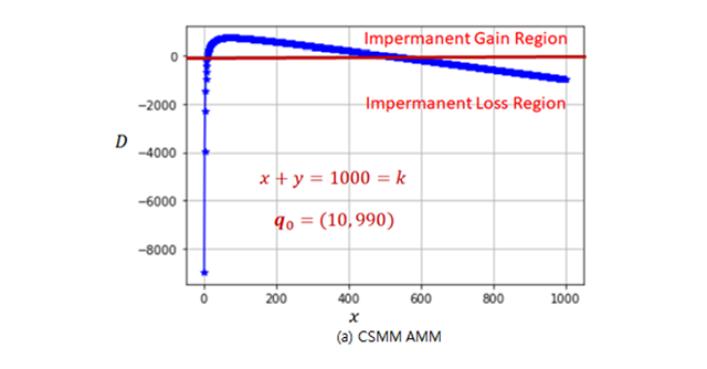
Figure 2(a) shows that impermanent gain occurs for a set of two

x_{0}

values. In this case, the asset cost function is

x + y

= 1000, and the initial asset pair is given as

q_{0}

= (10, 990), for example. The difference

D (x_{n})

is given as follows:

D = \frac{1}{x_{n}} [- 2 {x_{n}}^{2} + 1020 x_{n} - 10000]

(28)

Thus, for

x_{n}

= 10 or

x_{n}

= 500,

D (x_{n})

is zero, which states that this CSMM AMM system has no loss or gain at these points. For 10

< x_{0} <

500, the CSMM AMM has impermanent gain. Note that impermanent gain is innate in this case for the given initial asset pair. In Figure 2(a), at

x_{n}

= 10, zero crossing happens. Naturally,

x_{n}

is equal to

x_{0}

. However, at

x_{n}

= 500, another zero crossing happens. Thus, the left-hand side region from

x_{n}

= 10 is the impermanent loss region. Similarly, the right-hand side region from

x_{n}

= 500 is the impermanent loss region. The middle region between

x_{n}

= 10 and

x_{n}

= 500 is the impermanent gain region.

In this example, impermanent loss region and impermanent gain region coexist for all initial asset pairs

q_{0}

(x_{0}, y_{0})

except the value

x_{0}

= 500. The CSMM AMM with the initial asset pair, for example,

q_{0}

= (500, 500) and the asset cost function

x + y

= 1000, there is no impermanent gain region only in this condition. The existence of the impermanent gain region depends on the type of AMM, asset cost function with different constant

k

, and initial asset pair with different values of

x_{0}

C. Liquidity-Sensitive Logarithmic Market Scoring Rule

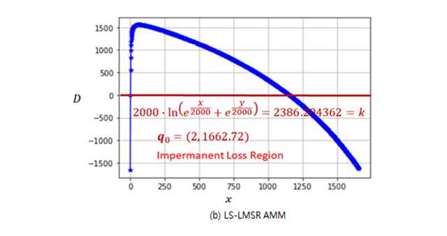
For the LS-LMSR, the value of

D (x_{n})

is a high-order function of

x_{n}

. Therefore, the closed-form solution cannot be easily derived, and we cannot show analytically whether this AMM has the property of impermanent loss or impermanent gain. Figure 2(b) shows an example of a situation similar to Figure 2(a). The asset cost function, in this case, is given as Equation (13), where

b

= 1000. For

q

= (1000, 1000), the value of

k

is 2386.294632. If the initial asset pair is

q_{0}

= (2, 1662.72), we can obtain Figure 2(b) that contains both impermanent loss and impermanent gain regions. Two zero crossings exist: one occurs at

x_{n}

= 2, and the other one is somewhere between

x_{n}

= 1154 and

x_{n}

= 1156. In this example, impermanent loss region and impermanent gain region coexist for all initial asset pair

q_{0}

(x_{0}, y_{0})

for the values

x_{0}

< 271.

Observation 2: If

x_{0} = y_{0}

, LS-LMSR AMM for Equation (11) has an impermanent loss property only for all

x_{n}

and

y_{n}

, which are both positive.

D. Constant Circle Market Maker

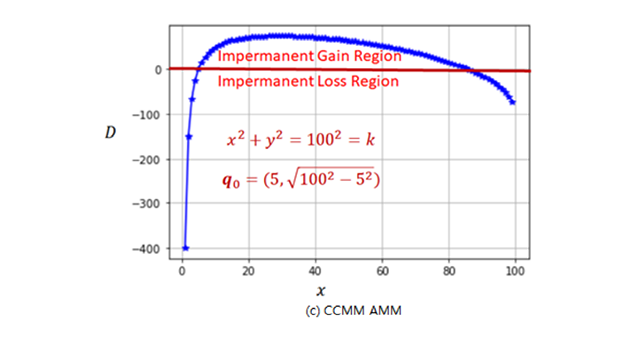
For the CCMM AMMs, the value of

D (x_{n})

is also a high-order function of

x_{n}

. Therefore, the closed-form solution cannot be easily derived, and we cannot show analytically whether this AMM has the property of impermanent loss or impermanent gain. Figure 2(c) shows an example of the situation similar to Figures 2(a) and 2(b).

The asset cost function, in this case, is given as Equation (18), where

a

= 0,

b

= 0, and

k

= 1002. For

q

= (100/√2, 100/√2), the value of

k

is 1002. If the initial asset pair is

q_{0}

= (5, 99.8749), we can obtain Figure 2(c) containing both impermanent loss and impermanent gain regions. Similarly, there are two zero crossings: one occurs at

x_{n}

= 5, and the other one is somewhere between

x_{n}

= 85 and

x_{n}

= 87. In this example, impermanent loss region and impermanent gain region coexist for all initial asset pair

q_{0}

(x_{0}, y_{0})

except the value

x_{0}

= 100/

\sqrt{2}

Appendix A shows the condition when the

D (x_{n})

has the property of impermanent loss only for the asset cost function

x^{2} + y^{2} = k

. Based on this simple case, we can derive the condition having both impermanent loss and impermanent gain property.

Observation 3: If

x_{0}

\frac{k}{\sqrt{2}} + a

, and

y_{0} = \frac{k}{\sqrt{2}} + b

, then CCMM AMM for Equation (18) has impermanent loss property only for all

x_{n}

and

y_{n}

, which are both positive.

IV. CONCLUDING REMARKS

This study reviews four constant function market makers: LS-LMSR, CPMM, CSMM, and CCMM. For the first time, this study showed the existence of impermanent gain mathematically and computationally thorough experiments. This paper showed that CPMM has impermanent loss property only. Meanwhile, LS-LMSR, CSMM, and CCMM can have both impermanent loss and impermanent gain altogether. For a specific condition, they have impermanent loss property only (see Observations in the previous section).
Even though an impermanent loss exists in CPMM AMM, this market maker attracted a large amount of total valued locked (TVL) and leads the decentralized exchange markets. Liquidity providers want impermanent gain rather than impermanent loss. The existence of impermanent gain will be fully exploited in the future DeFi systems. However, impermanent gain also has the problem. Liquidity providers want to withdraw the assets from the liquidity pool when impermanent gain occurs. When liquidity providers encounter impermanent gain, the liquidity provider earns extra profits in addition to the deposited assets. Thus, the liquidity providers are motivated to leave the pool, taking advantage of the assets they deposited and the kind of windfall profit that comes from impermanent gain. Meanwhile, impermanent loss makes the liquidity providers passive in joining the pool as they lose by depositing the asset, whereas impermanent gain makes the liquidity providers take extra profit and leave the pool. However, liquidity providers may prefer impermanent loss to impermanent gain. Whether liquidity providers will prefer impermanent loss or impermanent gain will be the subject of important research. A study on the attitudes of arbitrage traders in a market where impermanent loss and impermanent gain coexist would also be interesting.
It is well known that impermanent loss exists, but that impermanent gain is not. The reason is probably because the definition of divergence loss was not correct. In CSMM LP, it seems that further research has not been carried out by accepting the divergence loss as zero according to the wrong mathematical definition. Therefore, it seems that studies on divergence loss for LS-LMSR LP, etc., with more complex formulas have not been conducted. Since the existence of impermanent gain has been proven through examples in this paper, it is hoped that further research on impermanent gain will proceed in the future.

ACKNOWLEDGMENT

The authors would like to thank the anonymous reviewers for their time and effort to improve the quality of the paper by providing constructive comments.

REFERENCES

[1]	L. R. Abbade, F. M. Ribeiro, M. H. da Silva, A. F. P. Morais, E. S. de Morais, E. M. Lopes, A. M. Alberti, and J. Rodrigues, “Blockchain applied to vehicular odometers,” IEEE Network, vol. 34, no. 1, pp. 62-68, 2020.
[2]	G. Angeris and T. Chitra, “Improved price oracles: Constant function market makers,” Proceedings of the 2nd ACM Conference on Advances in Financial Technologies, pp. 81-90, 2020.
[3]	G. Angeris, A. Evans, and T. Chitra, “When does the tail wag the dog? Curvature and market making,” 2020. https://arxiv.org/pdf /2012.08040.pdf
[4]	G. Angeris, H.-T. Kao, R. Chiang, C. Noyes, and T. Chitra, “ An analysis of Uniswap markets, Cryptoeconomic Systems Journal, 2019. https://ssrn.com/abstract=3602203.
[5]	Z. Cui, F. Xue, S. Zhang, X. Cai, Y. Cao, W. Zhang, and J. Chen, “A hybrid blockchain-based identity authentication scheme for multi-WSN,” IEEE Transactions on Services Computing, vol. 13, no. 2, pp. 241-251, 2020.
[6]	M. Egorov, “StableSwap-efficient mechanism for stablecoin liquidity,” 2019. https://www.btcmoney.cc/uploads/ home/20200901/88eaf78993e5ab 93a5860afddc81fc74.pdf.
[7]	S. Eskandari, S. Moosavi, and J. Clark, “SoK: Transparent dishonesty: Front-running attacks on blockchain,” Third Workshop on Trusted Smart Contracts, 2019. http://fc19.ifca.ai/wtsc/ TransparentDishonesty.pdf.
[8]	A. Evans, “Liquidity provider returns in geometric mean transparent dishonesty: Front-running attacks on blockchain markets,” 2020. https://arxiv.org/pdf/2006.08806.pdf.
[9]	R. Hanson, “Combinatorial information market design,” Information Systems Frontiers, vol. 5, no. 1, pp. 107–119, 2003.
[10]	R. Hanson, “Logarithmic markets coring rules for modular combinatorial information aggregation,” The Journal of Prediction Markets, vol. 1, no. 1, pp. 3–15, 2007.
[11]	H. J. Kim, S. Choi, Y. T. Yoon, and S. Yoo, “Impermanent loss and gain of automatic market maker smart contracts,” 2022. https://www.techrxiv.org/articles/ preprint/Impermanent_Loss_and_Gain_of_ Automated_Market_Maker_Smart _Contracts/19196960.
[12]	B. Krishnamachari, Q. Feng, and E. Grippo, “Dynamic curves for decentralized autonomous cryptocurrency exchanges,” 2021. https://arxiv.org/pdf/2101.02778.pdf.
[13]	A. Kumari, R. Gupta, S. Tanwar, S. Tyagi and N. Kumar, "When blockchain meets smart grid: Secure energy trading in demand response management," IEEE Network, vol. 34, no. 5, pp. 299-305, 2020.
[14]	K. Lee, J. I. James, T. G. Ejeta, and H. J. Kim, “Electronic voting service using blockchain,” Journal of Digital Forensics, Security and Law, vol. 11, no. 2, pp. 123-135, 2016.
[15]	Z. Li, J. Kang, R. Yu, D. Ye, Q. Deng, and Y. Zhang, “Consortium blockchain for secure energy trading in industrial internet of things,” IEEE Transactions on Industrial Engineering, vol. 14, no. 8, pp. 3690- 3700, 2018.
[16]	F. Martinelli and N. Mushegian. “Balancer: A non-custodial portfolio manager, liquidity provider, and price sensor,” 2019. https://balancer.finance/whitepaper.
[17]	A. Othman, Automated Market Making: Theory and Practice, PhD Dissertation, Carnegie Mellon University, 2012.
[18]	A. Othman, D. M. Pennock, D. M. Reeves, and T. Sandholm, “A practical liquidity-sensitive automated market maker,” ACM Transactions on Economics and Computation, vol. 1, no. 3, pp. 1–25, 2013.
[19]	N. Tiruviluamala, A. Port, and E. Lewis, “A general framework for impermanent loss in automated market makers,” 2022. https://arxiv.org/abs/2203.11352.
[20]	M Turkanović, M. Hölbl, K Košič, M Heričko, and A Kamišalić, “EduCTX: A blockchain-based higher education credit platform,” IEEE Access, vol. 6, pp. 5112-5127, 2018.
[21]	Y. Wang, “Automated market makers for decentralized finance (DeFi),”https://arxiv.org/pdf/20 09.01676.pdf.
[22]	S. Wang, L. Ouyang, Y. Yuan, X. Ni, X. Han, and F.-Y. Wang, “Blockchain-enabled smart contracts: Architecture, applications, and future trends,” IEEE Transactions on Systems, Man, and Cybernetics, vol. 49, no. 11, pp. 2266-2277, 2019.
[23]	Y. Yuan and F.-Y. Wang, “Blockchain and cryptocurrencies: Model, techniques, and applications,” IEEE Transactions on Systems, Man, and Cybernetics, vol. 48, no. 9, pp. 1421-1428, 2018.

APPENDIX A

For the CCMM asset cost function

{x_{n}}^{2} + {y_{n}}^{2} = k

D (x_{n})

is given from Equation (21) as follows:

D (x_{n}) = 2 y_{n} - (\frac{y_{n}}{x_{n}} x_{0} + y_{0})

The condition that

D (x_{n})

is to be zero is given as

2 y_{n} x_{n} - y_{n} x_{0} - y_{0} x_{n} = 0

2 y_{n} x_{n} - y_{n} x_{0} = y_{0} x_{0}

where

y_{n} = \sqrt{k - {x_{n}}^{2} \geq 0}

and hence,

2 \sqrt{k - {x_{n}}^{2} x_{n}} - \sqrt{k - {x_{n}}^{2} x_{0}} = y_{0} x_{n}

{(2 \sqrt{k - {x_{n}}^{2} x_{n}} - \sqrt{k - {x_{n}}^{2} x_{0}})}^{2} = {(y_{0} x_{n})}^{2}

- 4 {x^{4}}_{n} + 4 x_{0} {x_{n}}^{3} + (4 k - {x_{0}}^{2}) {x_{n}}^{2} - 4 k x_{0} x_{n} + k {x_{0}}^{2} = {y_{0}}^{2} {x_{n}}^{2}

The left-hand side of the equation is a fourth-order polynomial open downward, whereas the right-hand side is a quadratic polynomial open upward. Thus, the following three possibilities exist:

1. When both side polynomials do not meet, then the right-hand side polynomial has larger value for all $x_{n}$ , and thus, $D (x_{n})$ is negative. It means that the AMM has the property of impermanent loss only.
2. When both side polynomials meet at a single point, then the situation is similar to the case of 1 (i.e., impermanent loss only).
3. When both side polynomials meet at more than a single point, then $D (x_{n})$ is either negative or positive, depending on the value of $x_{n}$ . It means that the AMM has the property of impermanent loss and impermanent gain altogether.

Hyoung Joong Kim is currently a professor at Korea University, Korea and the president of the Korea Fintech Society. He received his Ph.D. in Control and Instrumentation Engineering from Seoul National University, Korea. His main research areas are cryptocurrencies, decentralized finance and fintech security.

Soohyuk Choi is currently the CEO of SymVerse, a crypto company in Korea, and president of the Korea Blockchain Startup Association. He received his Ph.D. in Economics from Northwestern University, USA.

Yong Tae Yoon is currently a professor at Seoul National University, Korea and head of the Electric Power Research Institute. He received his Ph.D. in Electrical Engineering from MIT, USA.

Shiyong Yoo is currently a professor at Chung-Ang University, Korea. He received his Ph.D. in Applied Economics/Finance from Cornell University, USA

List